From Backprop to BPTT
A Hint of History
The Back-propagation Algorithm is, with no doubt, one of the most important and powerful mathematical tool used by a variety of machine learning models. Using the chain rule and partial derivative, it computes the gradient of the cost function with respect to each element in the weight matrix at each layer of the neural network. And this calculation informs us how fast the cost will change when we change the weights and biases within our network.
First proposed by Seppo Linnainmaa in 1970, back-propagtion was later introduced to train neural network in 1974 by Paul Werbos in his famous PhD dissertation. But the algorithm did not gain enough appreciation until a famous paper in 1986 by David Rumelhart, Geoffrey Hinton, and Ronald Williams, who achieved some breakthrough success in several supervised learning tasks.
Rumelhart and et al.’s paper, illustrating how back-propagation can adjust the weights of the network to better minimize the error between actual and desired output vectors, demonstrates the algorithm’s ability to create new features, work faster, and sovle problems that were “insoluble” by some earlier approaches, including the Perceptrons.
Not long after Rumelhart and et al.’s paper came out, a series of variants of the Backprop model were also invented, among which the most important ones are the Back-propagation Through Time (BPTT) by Pearlmutter in 1989, Epochwise BPTT, Truncated BPTT (TrBPTT), and Real Time Recurrent Learning (RTRL), well explained by Paul Webos in his another influential paper and Ronald Williams and David Zipser in their 1990 article.
In this post, I will illustrate how the simple, initial Backprop model evolves into the later BPTT and its variants, which further lay down a solid foundation for another powerful model: Long Short-Term Memory (LSTM). I will talk about LSTM in the next post.
- A History of History
- How Does Backpropagation Work?
- How Does BPTT Work?
- Epochwise and Truncated BPTT
- Real Time Recurrent Learning
How Does Backprop Work?
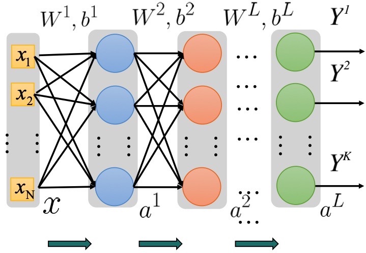
Figure 1. A simple fully connected network. (Image Source:)
Let us start with some basic math notations. The diagram above is a fully connected neural network with \(L-1\) hidden layers and the output layer \(a^{(L)}\). The input vector \(X\) is an \(N\)-by-\(1\) vector. \(W^{(i)}\) represents the matrix multiplied by the feedforward input at each layer \(i\), while \(b^{(i)}\) is a bias vector added at each hidden layer. \(a^{(i)}\) is an \(M\)-by-\(1\) vector storing each hidden neuron at layer \(i\). At last, \(Y^{(k)}\) represents the desired value of a single output unit \(k\) inside the \(K\)-by-\(1\) label vector(from the training samples). Note that in many cases, \(dim(a^{(i)})\) may not necessarily equals \(dim(X)\) and \(dim(a^{(i)})\) can vary throughout the layers.
At each layer \(i\), the feedforward input \(x^{(i)}\) or \(a^{(i)}\) was multiplied by its corresponding matrix \(W^{(i)}\) and added by the bias vector \(b^{(i)}\), and we denote this result as \(z^{(i)}\). This \(z^{(i)}\) will be then passed into a non-linear activation function \(f\) (often sigmoid or softmax) and gives the values of the hidden vector \(a^i\), which is fed forward as input for the next layer. Let’s dig in deeper into the math behind it.
At the \(1^{st}\) layer, we have:
At the \(2^{nd}\) layer, we have:
The equation writes similarly for the rest of the hidden layers. Then at the output layers, we can have:
Then, we would like to calculate the Total Error using Mean Squared Error (MSE) function \(E\) and sum up the errors over all the output nodes (About why using the MSE, see here),
where the first term is the MSE and the second one an optional regularization term.
**Important!** Keep in mind that our ultimate goal is to calculate \(\frac{\delta E}{\delta W_{ij}^{l}}\), the derivative of error function \(E\) with respect to an arbitrary element at row \(i\) and column \(j\) in an arbitrary matrix \(W^{(l)}\) at layer \(l\).
Denote the error of a single output unit \(k\) as:
As a result, the Total Error can be re-written as:
and its derivative as:
The rest of the job is then to calculate \(\frac{\delta H_k}{\delta W_{ij}^{l}}\). And we can decompose it as:
and denote:
Okay! Now let’s first start with an example to compute the derivative of \(H\) w.r.t the output unit \(i\) at the output layer \(L\) using the chain rule:
And we can use \(\delta^{(L)}\) to denote the error vector containing all these single output error. Bear in mind that this \(\delta^{(L)}\) is the term that will propagate backward into the network and help us calculate the derivatives of \(H\) w.r.t to the hidden units!
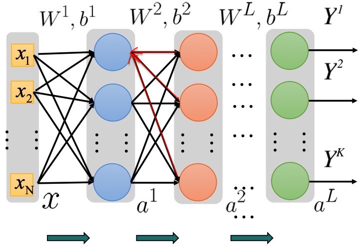
Now we can extend the the calculation of \(\delta_i^{(l)}\) to the hidden layers. Because the error flow is propagating backward(or leftward), we can write the equation for \(\delta_i^{(l)}\) in terms of the error from the next layer \(\delta^{(l+1)}\). (This, in fact, is Dynamic Programming)
This equation might seem frightening at first sight. However, as presented by the figure below, because \(\delta_i^{(l)}\) is influenced by errors propagating backward from all the units in the next layer, indicated by the red arrows, we will have to take all of these units into account, denoted \(\delta^{(l+1)}\). So the \(i^{th}\) row of the transpose of \(W^{(l+1)}\) will be the weights that the errors are moving through.
Nice! Then very simply:
Plugging eq.\((4)\) and \((5)\) back to the \((2)\) will give us the following:
Finally, if we plug in eq.\((6)\) back to (1), we will obtain the final equation for \(\frac{\delta E}{\delta W_{ij}^{l}}\), which will be used in gradient descent to update the weight at each training epoch:
How to train in Backpropagation?
We will use this wonderful GIF below to explain how to train a network using Back-propagation.
Figure 3. Forward and Backward Pass of Back-propagation(Image Source))
For each training sample from the dataset, say \(T_0\), we will feed the input vector into the network to perform a forward pass. After we obtain the predicted output, we will calculate the error(loss) function and perform a backward pass to update each weight in the matrix in each layer. After all weights are updated, we will then enter the next training epoch and feed in the next sample \(T_1\). The process repeats itself till we exhaust all training samples.
However, the training procedure in Backpropagation suffers from a major drawback termed catastrophic forgetting. This problem happens when a net having already learned the first training sample is then trained on the second sample, the new update of the weights may entirely erase the information previously learned. This gives rise to our next model, Backpropagation Through Time, which greatly resolves the problem of Backprop.